meandr allows for easy generation of coordinates that are random, yet continuously differentiable. This is particularly useful for simulating time-series measurements of physical phenomena that maintain a clear local trajectory.
Installation
devtools::install_github("sccmckenzie/meandr")Why meandr?
Suppose we want to simulate behavior of a “somewhat random” time-series phenomenon.
- Outdoor temperature
- Train station crowd density
- Stock price
Although we can’t predict the exact values of these examples, we know how they will behave to a certain extent. For instance, outdoor temperature is not going to drop by 100 degrees in 1 second.
We could use method #1 below:
method_1 <- data.frame(t = 1:100,
                       f = rnorm(100))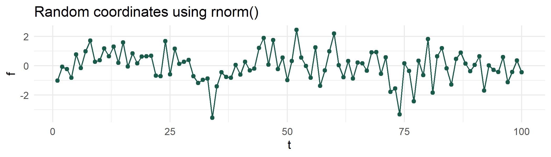
The above data doesn’t exhibit any prolonged directional consistency. This may not adequately emulate the character of the above examples.
meandr offers a solution to this problem. Each call to meandr() generates a unique tibble of t and f coordinates. For reproducibility, a seed argument is provided.
library(meandr)

df1 <- meandr(n_points = 100,
              n_nodes = 20,
              seed = 2)

df1
#> # A tibble: 100 x 2
#>         t        f
#>     <dbl>    <dbl>
#>  1 0.01   -0.00400
#>  2 0.02   -0.0160
#>  3 0.03   -0.0360
#>  4 0.04   -0.0640
#>  5 0.05   -0.100
#>  6 0.06   -0.144
#>  7 0.0700 -0.196
#>  8 0.08   -0.256
#>  9 0.09   -0.324
#> 10 0.10   -0.400
#> # ... with 90 more rows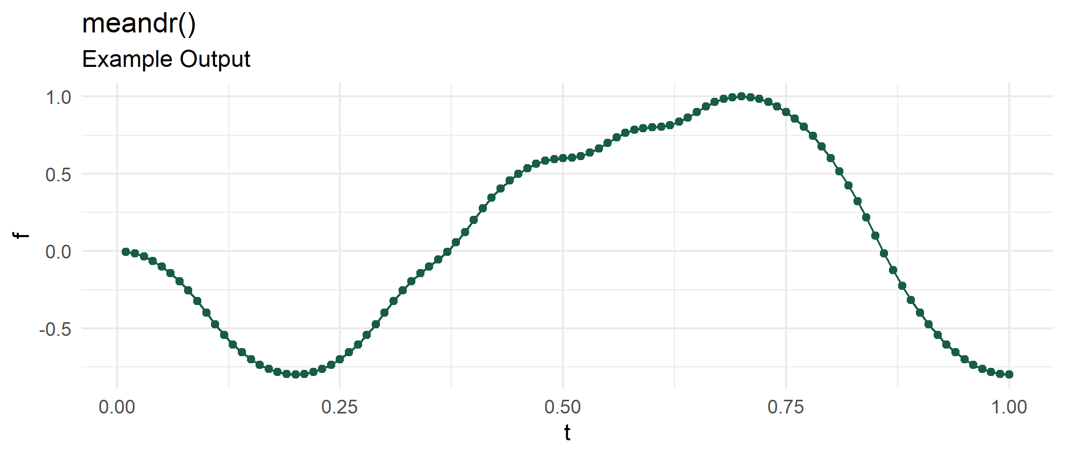
Observe df1 curve trajectory never radically changes between two points. This is a key feature of meandr: all curves are continuously differentiable.
