Generate random coordinates following continuous trajectory

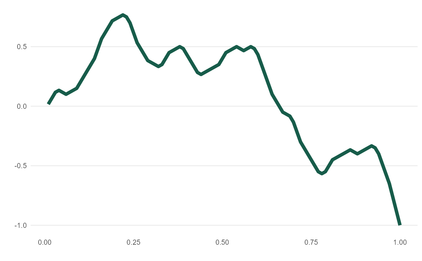
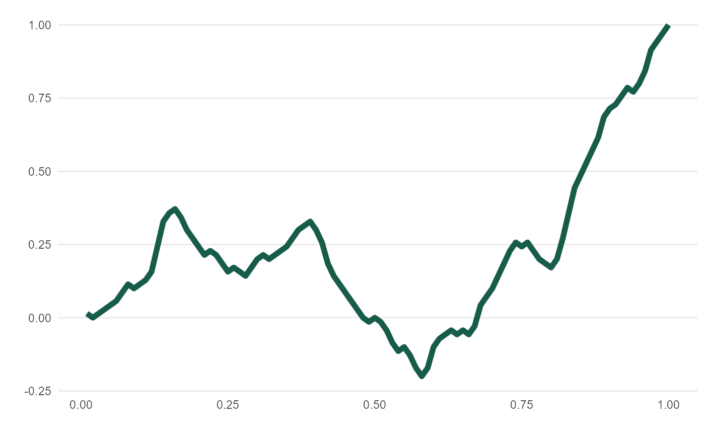
meandr() offers a calculus-driven approach to simulating random time-series behavior. Inputs n_nodes and wt serve as tuning knobs for overall smoothness and direction, respectively.

For greater control over curve shape, see create_path()

meandr(
  n_nodes = 100L,
  wt = c(1, -1),
  gain = 0.75,
  n_points = 100L,
  scale = 1,
  seed = NULL
)

Arguments

n_nodes	An integer. Defines number of distinct inflection points in function.
wt	A numeric vector of values. These will be sampled (with replacement) n_nodes times to create inflection points.
gain	Tuning parameter.
n_points	An integer. Controls output "resolution". (Underlying calculus is unaffected).
scale	A number. Adjusts all y-values so that max(y) = scale.
seed	A number passed to set.seed for repeatability. If NULL, no seed created.

Value

A tibble containing coordinates of resulting function.

Details

For wt, recommend using length 2 comprising of positive and negative element - though any numeric vector will be accepted. Default value, c(1, -1), will tend to produce curves with greatest directional variety. As magnitude between wt[1] and wt[2] deviates, overall curve will veer to +/- Inf.

Each call to meandr() follows below execution flow:
(1) Build piecewise function, "f2", of "nodes" sampled (with replacement) from wt.
(2) Integrate "f2" twice to obtain continuously differentiable function, "f".
(3) Interval (0, 1] is cut into n_points - resulting values passed to "f".
(4) Output coordinates in tibble

Examples

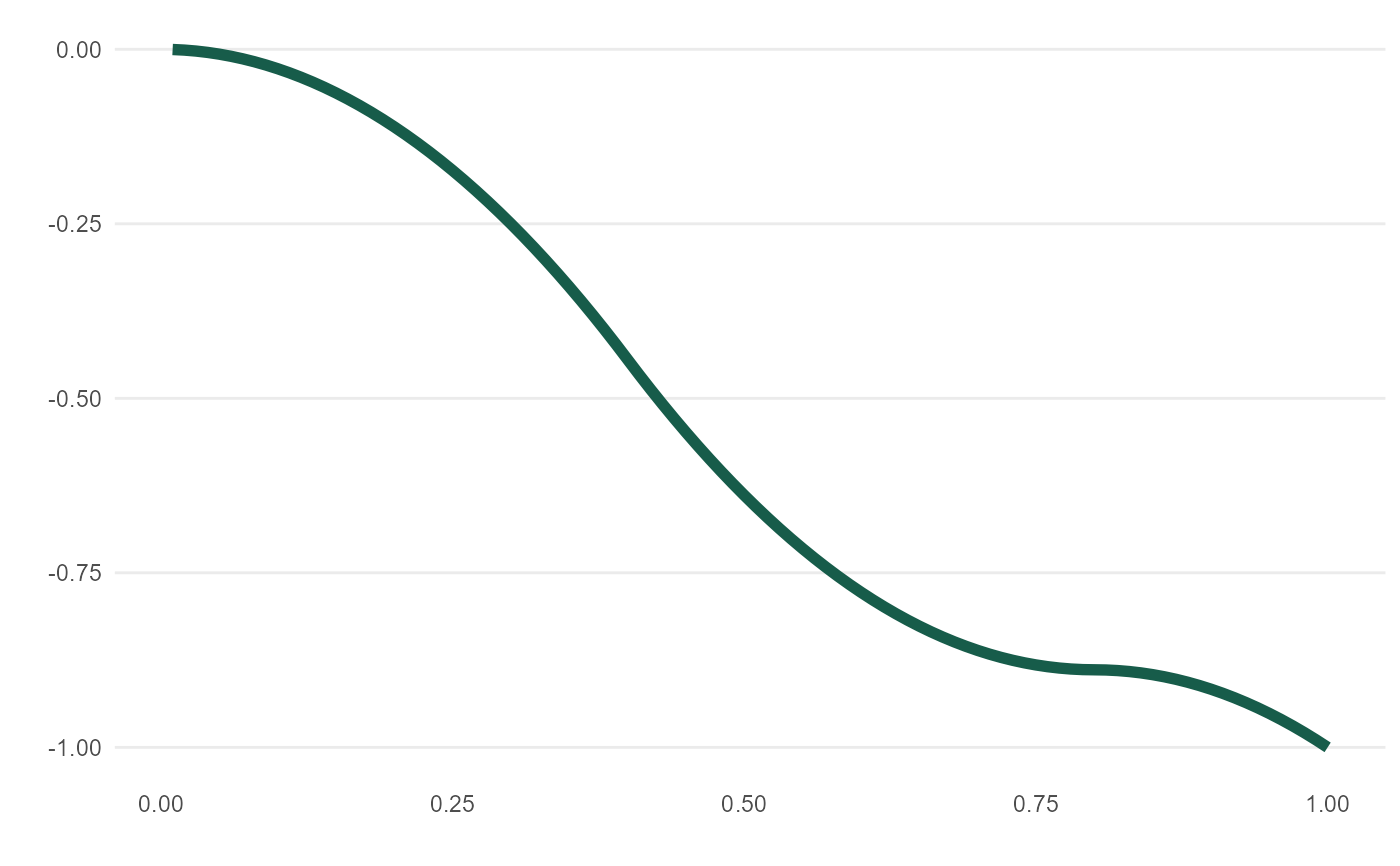
# See vignette("meandr")

# each call produces unique output
meandr()
#> # A tibble: 100 x 2
#>         t       f
#>     <dbl>   <dbl>
#>  1 0.01   -0.0313
#>  2 0.02   -0.125 
#>  3 0.03   -0.219 
#>  4 0.04   -0.25  
#>  5 0.05   -0.281 
#>  6 0.06   -0.313 
#>  7 0.0700 -0.344 
#>  8 0.08   -0.375 
#>  9 0.09   -0.344 
#> 10 0.10   -0.25  
#> # ... with 90 more rows

# use meandr::mplot for quick plotting
mplot(meandr())

# n_nodes has the most impact on curve complexity
curve1 <- meandr(n_nodes = 5)
mplot(curve1) # simple piecewise quadratic

curve2 <- meandr(n_nodes = 200)
mplot(curve2) # more meandering!